


Can math spot a future NFL bust better than a scout’s gut?
Analytical models that predict NFL draft busts try to do just that.
They turn combine numbers, college production, film grades, age and medical flags into clear probability buckets like Pro Bowler, Starter, Replacement, and Non-Factor.
Position-specific models and calibration techniques make those percentages meaningful.
My thesis: these frameworks give measurable risk signals that often match careers, but limits like small samples, missing validation, and noisy labels mean teams should use them as tools, not answers.
Core Predictive Frameworks Used in Analytical Models for NFL Draft Bust Identification

Public analytical models break prospects into discrete outcome buckets to measure bust risk. You’ll see five categories most often: Pro Bowler, Starter, Backup, Replacement, and Non-Factor. A 2026 class model shows this with real numbers. Fernando Mendoza gets a 0.5% non-factor chance and a combined 55.9% Pro Bowler/Starter probability. Drew Allar sits at 60.4% combined Replacement/Non-Factor. Carson Beck hits 58.9% in that same bucket. These aren’t abstract scores. They’re actionable risk profiles built from raw inputs.
Most systems use Pro Football Reference’s Approximate Value as the outcome label. That converts historical AV data into training targets that track career trajectory, not just one good season.
You’ll find model architectures all over the map. Logistic regression and penalized generalized linear models handle binary bust/non-bust calls. Tree-based methods like random forests and gradient boosting grab non-linear interactions. Ensemble approaches stack multiple algorithms to toughen up predictions. Bayesian hierarchical models pool data across positions and draft years when sample sizes get thin. Calibration techniques like reliability curves and Brier scoring convert raw outputs into probabilities you can actually trust. A forecasted 60% bust risk should pan out six times in ten over the long haul.
Several public tools don’t publish historical accuracy rates, cross-validation protocols, or error metrics. That limits external validation, but it doesn’t kill the underlying signal.
Fundamental model inputs:
• Athletic testing from the NFL Combine and Pro Days (40-yard dash, three-cone drill, broad jump, bench press reps, vertical jump, shuttle run)
• College production adjusted for strength of schedule and opponent quality
• Age relative to draft class and years of college starting experience
• Film-derived grading and advanced tape metrics
• Injury history and medical red flags from team physicals
• Consensus big board rankings from aggregated scouting services
High replacement/non-factor percentages work as practical bust indicators. They bundle the model’s expectation that a prospect contributes minimally or leaves the league early. When a quarterback’s combined Replacement/Non-Factor probability crosses 50–60%, you’re looking at outcomes that cluster in low-impact or short-tenure territory. Drew Allar’s 60.4% and Carson Beck’s 58.9% both clear this line. That marks them as high-risk picks even if consensus rankings put them in the first or second round. Teams using these models treat those probabilities as red flags. They dig deeper on transferable skills, scheme fit, and intangibles before committing draft capital to prospects the algorithm tags as probable busts.
Feature Engineering Approaches for NFL Draft Bust Prediction Models
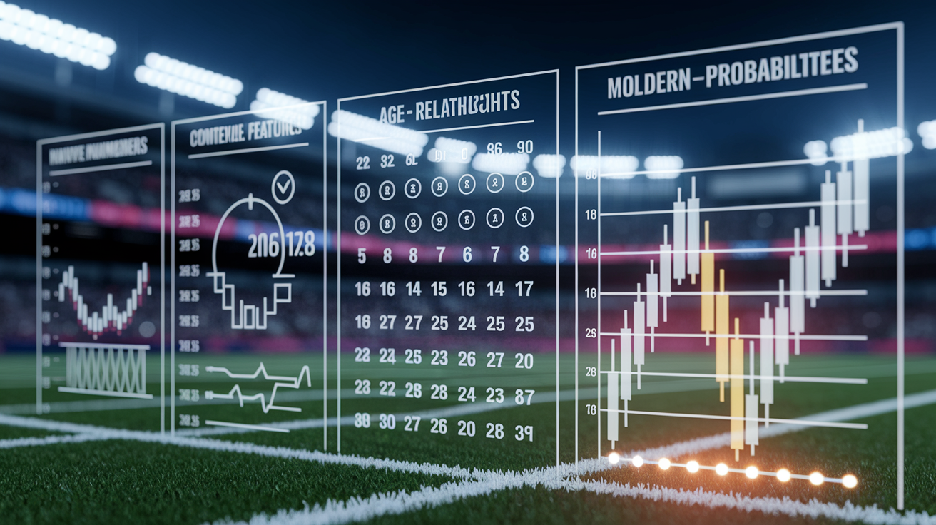
Raw measurements only gain predictive power after you transform them into contextual, normalized, interaction-rich features. Standard practices include age-relative-to-class normalization, which compares a prospect’s birthdate to the median age of peers at the same position. Opponent-adjusted production statistics weight college output by the quality of defenses faced. Analysts also compute variance in college game grades as a volatility proxy. Low week-to-week variance suggests consistency. High variance flags boom-or-bust risk.
Market-implied probabilities from betting odds bring real-time aggregated information. When a prospect’s draft-position prop line drifts from 1.50 to 4.00, the shift might encode medical flags or interview failures not yet public. Interaction terms capture synergies between features. Size × athleticism × positional archetype interactions don’t show up in univariate metrics.
Engineered metrics that improve bust prediction:
- Market-implied probability signals pulled from betting-market odds movements and consensus line shifts
- Age-relative-to-class normalization that penalizes older prospects who benefited from physical maturity advantages in college
- Opponent-adjusted production statistics weighted by strength of schedule and conference-level defensive efficiency
- Volatility proxies computed as the standard deviation of per-game grading or the range between ceiling and floor performances
- Interaction terms between height, weight, athleticism, and position-specific archetypes
Positional differences demand tailored feature sets. Quarterback models prioritize accuracy metrics under pressure, time-to-throw consistency, and cognitive processing speed inferred from pre-snap adjustment frequency. Offensive linemen require length-adjusted strength ratios and sustained-block win rates, not explosive short-area quickness. Wide receivers benefit from separation metrics at stem points and contested-catch conversion rates. Edge rushers get evaluated on bend ability, hand usage efficiency, and pressure rate against varying protection schemes.
A one-size-fits-all feature set dilutes signal. It forces the algorithm to learn positional nuances from scratch. Position-specific engineering bakes domain knowledge directly into the input layer. That raises ceiling accuracy and improves interpretability for scouts integrating model outputs with film study.
Machine Learning Algorithms Used to Predict NFL Bust Outcomes

Tree-based models dominate because they handle non-linear relationships, categorical variables, and missing data without extensive preprocessing. Random forests train multiple decision trees on bootstrapped samples and average predictions to reduce variance. Gradient boosting machines sequentially correct errors from prior iterations to minimize bias.
Published models explicitly report using random forests trained separately for each position. That lets the algorithm discover position-specific interaction patterns without cross-contamination from other roles. Neural networks offer additional flexibility through deep architectures that learn hierarchical feature representations. But they need larger training sets and careful regularization to prevent overfitting when historical draft data spans only a few hundred prospects per position. Ensemble stacking combines predictions from multiple algorithm families (trees, linear models, and neural nets) into a meta-model that captures complementary strengths.
| Algorithm | Strength | Weakness |
|---|---|---|
| Random Forest | Robust to overfitting; captures non-linear interactions without manual specification; handles missing data natively | Can underperform on extrapolation tasks; less interpretable than single trees; requires tuning of tree count and depth |
| Gradient Boosting | High predictive accuracy; sequentially reduces bias; flexible loss functions for imbalanced classes | Prone to overfitting if learning rate and iteration count not carefully controlled; slower training; sensitive to noisy labels |
| Neural Networks | Learns complex hierarchical representations; scales with data volume; can incorporate unstructured inputs like text or video embeddings | Requires large sample sizes; difficult to interpret; hyperparameter tuning is computationally expensive; risk of overfitting small datasets |
Position-specific modeling beats universal approaches because development timelines, relevant predictors, and outcome distributions vary dramatically across roles. Offensive tackles and defensive linemen mature slowly. They need three to four years before peak performance. Wide receivers and cornerbacks contribute immediately or wash out quickly. A quarterback’s bust risk hinges on processing speed and accuracy stability. Those variables mean nothing for a safety’s projection.
Training a single model across all positions forces the algorithm to allocate capacity to learning positional distinctions rather than refining within-position predictions. Separate models per position allow targeted feature selection, class-weight tuning for position-specific outcome base rates, and threshold calibration that reflects how teams actually deploy each role. This architecture mirrors how NFL front offices organize scouting departments by position coach. It embeds domain structure directly into the statistical framework.
Position-Specific Risk Models and Volatility Indicators
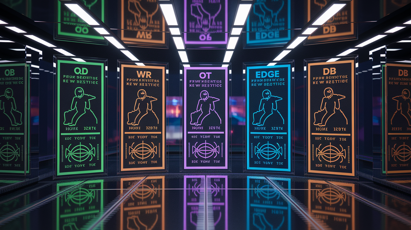
Premium positions (quarterback, edge rusher, offensive tackle, and wide receiver) show higher volatility because their impact on wins is large and their skill translation from college to NFL is uncertain. A low-volatility profile looks like an offensive lineman from a Power Five conference with three years of starting experience, stable technique grades, and measurables clustering near positional medians.
High-volatility prospects include project quarterbacks with limited tape, converting college athletes transitioning to new positions, and small-school edge rushers whose production came against weak competition. Volatility itself isn’t good or bad. It quantifies the range of plausible outcomes. Teams drafting in the top five minimize volatility to secure foundational pieces. Teams picking in the third round accept higher variance to chase upside at lower cost.
Position-specific predictors that improve bust classification:
• Quarterback accuracy stability across down-and-distance situations and pressure rates
• Wide receiver separation metrics at stem points, route-tree diversity, and contested-catch win rates
• Offensive tackle length-adjusted strength, anchor ability against bull rushes, and recovery speed after initial contact
• Edge rusher bend ability around the arc, hand-usage efficiency, and pressure rate normalized by opponent pass-block quality
• Defensive back ball production (interceptions, pass breakups) adjusted for target rate and coverage responsibility
Real prospect examples show these principles in action. Drew Allar’s 60.4% replacement/non-factor probability and Carson Beck’s 58.9% mark both flag high quarterback bust risk. Consensus rankings might place them in early rounds anyway. The models identify accuracy inconsistencies, limited processing speed under pressure, or physical tools that don’t translate to NFL timing.
Malaki Starks and Caleb Downs (top safeties Thieneman and McNeil-Warren in the scraped data) show very low bust rates. Safety is a lower-volatility position with clearer skill translation and less dependence on rare cognitive traits. Ty Simpson’s 46.9% combined Pro Bowler/Starter probability against only 17% replacement/non-factor risk represents a high-upside profile. The model sees genuine star potential balanced against modest downside. That’s a portfolio allocation attractive to teams willing to bet on developmental ceiling.
Case Study: Using Real Prospect Outputs to Understand Bust Probability
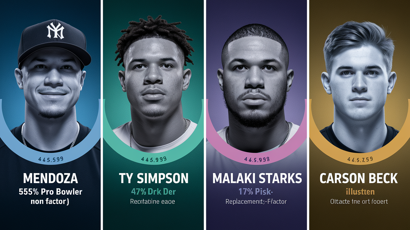
Fernando Mendoza’s probability distribution (27.9% Pro Bowler, 28.0% Starter, 0.5% Non-Factor) shows a prospect the model views as a near-certain NFL contributor with legitimate star upside. The combined 55.9% Pro Bowler/Starter rate signals high confidence in positive outcomes. The vanishingly small 0.5% non-factor chance suggests minimal downside risk.
Ty Simpson’s 46.9% combined Pro Bowler/Starter probability paired with only 17% replacement/non-factor risk presents a different shape. Meaningful upside with a floor that remains above replacement level. Both profiles justify first-round investment because the probability mass concentrates in productive outcome bins.
Drew Allar and Carson Beck tell the opposite story. Allar’s 60.4% replacement/non-factor combined probability means the model expects a majority of future scenarios to end with minimal NFL impact or a short career. Beck’s 58.9% in the same bucket reinforces high bust risk. When more than half of a prospect’s probability distribution sits in the two lowest outcome categories, teams face a coin flip between a marginal backup and outright failure. That matters because draft capital is finite. Spending a top-50 pick on a 60% bust-risk quarterback sacrifices the opportunity to select a player with a more favorable distribution.
The scraped recommendation to re-evaluate model performance after three years reflects the temporal lag required to measure career outcomes. Rookie-season statistics mislead because development curves vary by position and situation. A three-year window captures whether a prospect secured a starting role, maintained it, and generated surplus value relative to contract cost. Models demonstrating calibration at this horizon (where 60% bust forecasts materialize as actual busts in six of ten cases) earn credibility for future draft cycles.
Lessons these prospects illustrate:
- Upside concentration: When Pro Bowler and Starter probabilities combine above 50%, the model sees legitimate foundational talent worth early capital.
- Downside red flags: Replacement/Non-Factor probabilities exceeding 50–60% mark high bust risk that should trigger deeper diligence or position reassignment on the draft board.
- Volatility signatures: Wide probability spreads across all five bins indicate uncertain projection. Narrow spreads around Starter or Backup bins suggest safer floor with limited ceiling.
- Model uncertainty: Prospects with near-equal probabilities across three or more categories reveal insufficient data or conflicting signals. That warrants additional scouting investment before selection.
Data Sources, Cleaning Challenges, and Sample Bias in NFL Bust Models
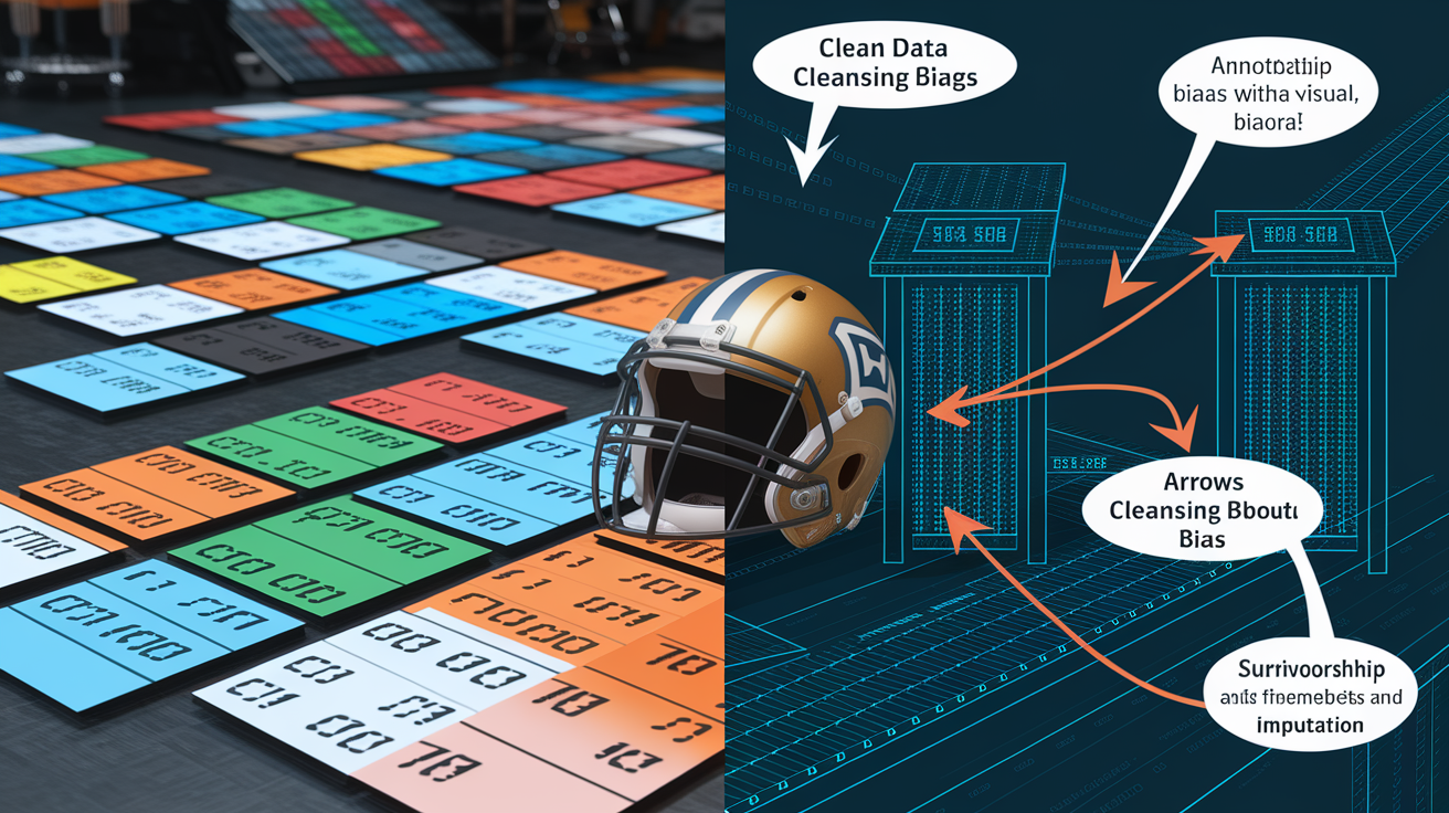
Most public models restrict their sample to NFL Scouting Combine invitees. That introduces survivorship bias by excluding small-school prospects, late-bloomers, and players who skipped the Combine for medical or strategic reasons. About 318 prospects attend each year’s Combine, but Pro Days generate additional measurements for hundreds more athletes. Models that ignore Pro Day-only participants underrepresent developmental archetypes and late-declared underclassmen.
Pro Day inflation issues compound this problem. Hand-timed 40-yard dashes run 0.08 to 0.12 seconds faster than electronic Combine times on average. Pro Day broad jumps often exceed Combine marks by several inches due to favorable conditions, custom surfaces, and selection bias in which drills athletes choose to repeat.
Missing data pervades draft datasets. Injury histories are incomplete because teams guard medical records closely. Interview scores and character evaluations remain proprietary. Some prospects skip specific drills. Standard imputation methods (mean substitution, regression-based fills, or multiple imputation) introduce noise when missingness isn’t random. A player who skips the bench press may do so because of a shoulder injury. That makes his missing value informative, not arbitrary. Sophisticated models use missingness indicators as separate features to capture this signal rather than discarding or blindly filling gaps.
Survivorship bias distorts long-term Approximate Value labeling because players who exit the league early generate low AV totals that may understate their true talent if injuries or coaching changes derailed development. Late-round picks who never receive a fair opportunity to start accumulate zero AV despite possessing starter ability. That biases the model to undervalue prospects from weak college programs or non-premier positions. Sample size limitations restrict position-specific models. Tight ends and fullbacks may have fewer than 50 draftees per year. That forces analysts to pool multiple draft classes and risks era effects from rule changes or positional usage trends.
| Issue | Effect | Mitigation |
|---|---|---|
| Combine-only sample restriction | Excludes small-school and Pro Day-only prospects; underrepresents developmental archetypes | Adjust Pro Day measurements using empirically derived correction factors; expand sample to include all drafted players |
| Pro Day inflation | Overestimates athleticism for prospects who skip Combine; introduces measurement inconsistency | Apply position-specific deflators to hand-timed 40s and self-selected drill results; flag Pro Day-only data with indicator variables |
| Missing data on injuries and interviews | Loses predictive signal; imputation introduces noise if missingness is informative | Create missingness indicators; use multiple imputation methods; integrate proprietary team data when available |
| Survivorship bias in AV labeling | Penalizes injury-shortened careers and situational non-starters; distorts outcome distributions | Censor observations at injury events; model opportunity-adjusted production; use alternative outcome metrics like starter designation |
| Small sample sizes for non-premium positions | Increases model variance; risks overfitting; limits power to detect rare predictors | Pool multiple draft years; apply hierarchical Bayesian models; use position groups rather than individual positions |
Evaluating Model Accuracy, Calibration, and Overfitting Prevention
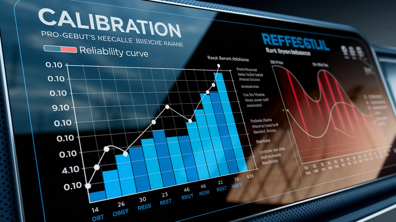
Cross-validation protocols separate historical draft data into training and holdout sets to estimate out-of-sample performance. K-fold cross-validation partitions the dataset into k subsets, trains on k-1 folds, and tests on the remaining fold. You repeat k times and average results. Temporal splits work better. Train on drafts from 2000–2015 and test on 2016–2020. That simulates real-world deployment where models forecast future classes.
Nested cross-validation tunes hyperparameters on an inner loop while evaluating final performance on an outer loop. That prevents information leakage from the test set into model selection. Without rigorous validation, you can’t tell genuine predictive signal from overfitting to historical noise.
Calibration measures whether forecasted probabilities match realized frequencies. A well-calibrated model that assigns 40% bust probability to 100 prospects should see about 40 of them actually bust. Reliability curves plot predicted probabilities against observed outcome rates. Perfect calibration follows the 45-degree diagonal. Systematic deviations reveal over- or under-confidence.
The Brier score quantifies calibration by computing the mean squared error between predicted probabilities and binary outcomes. It penalizes both poor discrimination and miscalibration. A Brier score of 0.10 in a binary classification task indicates strong performance. Scores above 0.25 suggest the model adds limited value over baseline rates.
Rare-event imbalance distorts classification thresholds when Pro Bowler outcomes occur in fewer than 5% of cases. Standard algorithms optimize overall accuracy. You can achieve 95% by predicting “not a Pro Bowler” for every prospect while completely failing to identify the rare stars. Class-weighting techniques penalize misclassification of the minority class more heavily. That shifts the decision boundary to improve recall on rare positives.
Precision-recall curves and area under the receiver operating characteristic curve (AUC-ROC) offer threshold-independent performance summaries. AUC values above 0.75 indicate useful separation between busts and hits. Some public models lack published calibration plots, backtests, or AUC metrics. That limits external validation and raises concerns about selective reporting of favorable results.
Integrating Scouting, Analytics, and Market Signals Into Bust Prediction Systems

Betting market odds aggregate dispersed information from sharp bettors, insiders, and informed observers. When a prospect’s draft-position prop line drifts from 1.50 (implied 67% probability of going in the top 10) to 4.00 (implied 25% probability), the shift often encodes medical red flags, poor interview performance, or character concerns that statistical models can’t capture from public data.
Market-implied probabilities extracted from these lines serve as real-time Bayesian priors that update model forecasts as new information arrives. A sudden odds collapse two days before the draft may signal a failed physical or off-field incident. That prompts teams to downgrade the prospect regardless of algorithmic output.
Human elements resist quantification but drive bust outcomes. Interview performance reveals cognitive processing speed, coachability, and maturity that combine measurables can’t detect. Character flags (prior suspensions, substance abuse history, or confrontational behavior) predict off-field incidents that end careers prematurely. Scheme fit determines whether a prospect’s college role translates to NFL responsibilities. A zone-blocking offensive lineman may struggle in a gap-scheme system. A press-man cornerback fails in soft zone coverage. These variables are auditable only through direct observation and interpersonal evaluation, not statistical inference.
Human-scouted red flags that elevate bust risk:
• Character concerns including prior team suspensions, substance abuse violations, or legal incidents that suggest immaturity or poor decision-making
• Coachability issues identified during interviews when prospects deflect criticism, lack self-awareness, or demonstrate fixed mindsets resistant to development
• Scheme fit mismatches where college role and responsibility don’t align with NFL team’s offensive or defensive system
• Medical red flags from pre-draft physicals revealing degenerative conditions, unreported injuries, or anatomical abnormalities that shorten career longevity
Odds-movement signals offer a practical bridge between scouting and analytics. A model that assigns 30% bust risk to a quarterback may raise that forecast to 50% if betting markets push the prospect’s draft position down three rounds in 48 hours. This integrated approach treats quantitative probabilities as baseline estimates that qualitative information (market moves, interview feedback, medical updates) can adjust in real time.
Teams using this framework avoid the false choice between “trust the model” and “trust the scouts.” They build decision systems where both inputs contribute complementary signals that reduce overall uncertainty and improve draft-day accuracy.
Building and Deploying Bust Prediction Tools for Front Offices

Front-office decision tools translate model probabilities into actionable draft-board rankings and trade-value calculations. Surplus Value (defined as player production minus rookie contract cost) serves as the primary optimization target because draft capital is scarce and teams maximize win probability per dollar spent. A quarterback on a rookie deal who performs as a league-average starter generates $20–30 million in annual surplus value compared to signing a veteran at market rate.
Bust prediction models feed directly into Surplus Value forecasts by weighting expected production by the probability of each outcome bin. A prospect with 60% bust risk generates far less expected surplus than one with 70% starter probability, even if their ceiling outcomes are identical.
Portfolio construction principles guide draft-class assembly. Teams balance low-volatility foundational picks (offensive linemen with three years of starting tape and stable technique) against high-variance upside gambles in the middle rounds where cost is lower. A first-round edge rusher with a narrow Starter/Backup probability distribution anchors the class. A fourth-round developmental quarterback with 30% Pro Bowler upside and 40% bust risk offers lottery-ticket value.
Published models that restrict their top 32 prospects to premium positions (QB, WR, OT, EDGE, DT, CB) reflect this portfolio logic. Non-premium roles like safety and inside linebacker deliver lower expected surplus even when projection confidence is high.
Front-office dashboard features that operationalize bust prediction:
- Probability distributions for each prospect across all five outcome bins (Pro Bowler, Starter, Backup, Replacement, Non-Factor) with visual heatmaps to quickly identify risk profiles
- Comparable player charts matching current prospects to historical players with similar measurables, production, and probability distributions to ground projections in concrete examples
- Surplus Value tables computing expected production weighted by outcome probabilities and subtracting positional rookie contract costs at each draft slot
- Decision thresholds calibrated to team strategy. Risk-averse teams drafting foundations in the top 10 set bust-risk maximums at 30%. Aggressive teams in later rounds accept 50% thresholds for upside plays.
- Head-to-head comparison modules allowing side-by-side evaluation of two prospects with different risk-return profiles to inform board ordering and trade decisions
Final Words
In the thick of it, we ran through core frameworks (logistic, tree-based, ensemble), feature engineering, machine learning choices, position-specific risk, and real prospect outputs.
We flagged data pitfalls like Pro Day inflation, survivorship and sample bias, missing calibration, and the need to retest models after a 3-year outcome window. You saw which inputs and engineered metrics matter and why 50–60% replacement/non-factor rates are a red flag.
If you’re evaluating or building analytical models that predict NFL draft busts, keep models transparent, position-aware, and well-calibrated. Do iterative backtests and fold in scouting signals. That makes forecasts actually useful and helps teams pick smarter.
FAQ
Q: How accurate is Mel Kiper?
A: Mel Kiper’s accuracy is mixed: he’s a long-standing draft analyst with useful context, but year-to-year accuracy varies by position; treat his rankings as informed guidance, not guaranteed predictions.
Q: What is the AI that predicts NFL games?
A: There isn’t a single AI that predicts NFL games; teams and companies use many methods—statistical models, random forests, gradient boosting, neural nets and ensembles—to forecast outcomes, with widely varying accuracy.
Q: What QB is Mr. Irrelevant?
A: The QB called Mr. Irrelevant is the quarterback selected with the NFL Draft’s final pick; the actual name changes yearly, so check the current draft list to see who holds that title.
Q: Who is the most accurate fantasy football analyst?
A: No single fantasy analyst is always the most accurate; accuracy depends on format and season. Analysts like Matthew Berry, Jamey Eisenberg, and consensus rankings tend to perform well—use multiple sources.